
a generic tool for stochastic DALY calculation in R
Sensitivity analysis studies how the uncertainty in the overall DALY estimate can be apportioned to the different sources of uncertainty in the input parameters. These results can therefore help to identify those input parameters that cause significant uncertainty in the overall DALY estimate and that therefore may be the focus of further research for reducing the overall uncertainty in the DALY estimate.
Implementation
The sensitivity() function implements a probabilistic global sensitivity analysis of the overall DALY estimate, in which the analysis is conducted over the full range of plausible input values (hence global), determined by the specified uncertainty distributions (hence probabilistic). Two general methods are available, i.e., based on (standardized) regression coefficients (method = "src") or on partial correlation coefficients (method = "pcc").
The sensitivity() function is defined as follows:
sensitivity(x, method = c("src", "pcc"), rank = FALSE, mapped = TRUE)
Specifying method = "src" will perform a linear regression-based sensitivity analysis. Here, the simulated overall DALY estimates will be regressed against the simulated values for the stochastic input parameters (using lm()). To facilitate comparison, the independent terms are standardized such that they are normally distributed with mean zero and standard deviation one (using scale()). The resulting regression coefficients are therefore referred to as standardized regression coefficients.
Argument rank specifies whether the regression should be performed on the actual values (rank = FALSE; default) or on the ranked values (rank = TRUE). Rank-based regression may be preferred when the relation between output and inputs is non-linear. As a rule of thumb, R^2 values smaller than 0.60 may be indicative of a poor fit of the default linear regression model.
If mapped = TRUE, the dependent term is not standardized, such that the resulting mapped regression coefficients correspond to the change in overall DALY given one standard deviation change in the corresponding input parameter. If mapped = FALSE, the dependent term is standardized, such that the resulting standardized regression coefficients correspond to the number of standard deviations change in overall DALY given one standard deviation change in the corresponding input parameter.
Specifying method = "pcc" will calculate partial correlation coefficients for each of the input variables. Partial correlation coefficients represent the correlation between two variables when adjusting for other variables. In the presence of important interactions between input variables, partial correlation coefficients may be preferred over standardized regression coefficients.
Argument rank specifies whether the correlation should be calculated between the actual values (rank = FALSE; default) or between the ranked values (rank = TRUE).
The sensitivity() function returns an object of class 'DALY_sensitivity'. Both a print() and plot() method are available for this class, the latter generating a tornado plot of the regression or partial correlation coefficients.
Example
For example, a sensitivity analysis of the Neurocysticercosis model, based on mapped standardized regression coefficients, could be performed as follows:
set.seed(123)
x <- getDALY(aw = TRUE, dr = 0.03)
sa <- sensitivity(x, method = "src", mapped = TRUE)

## show results of sensitivity analysis
print(sa)
Mapped standardized regression coefficients:

          Estimate Std. Error  t value  Pr(>|t|)

mrt1     21902.003      8.015 2732.596         0 ***
DWn1.3    1736.451      8.014  216.674         0 ***
DWn1.2     891.846      8.015  111.273         0 ***
DWt1.3     398.369      8.016   49.699         0 ***
inc1.F.3   288.485      8.015   35.995 5.76e-275 ***
inc1.M.3   275.811      8.016   34.409 4.09e-252 ***
DWn1.4     259.261      8.016   32.342 1.02e-223 ***
DWt1.2     201.790      8.015   25.177 9.97e-138 ***
DWn1.1     159.864      8.013   19.950  1.07e-87 ***
inc1.M.2   149.588      8.014   18.665  4.29e-77 ***
inc1.F.2   144.769      8.014   18.064  2.29e-72 ***
DWn1.5     100.915      8.014   12.593  3.17e-36 ***
trt1       -72.530      8.013   -9.051  1.54e-19 ***
DWt1.4      52.205      8.014    6.514  7.47e-11 ***
inc1.M.4    37.124      8.015    4.632  3.65e-06 ***
DWt1.1      35.729      8.014    4.458  8.31e-06 ***
inc1.F.4    33.616      8.015    4.194  2.75e-05 ***
inc1.F.1    21.062      8.014    2.628   0.00859 **
inc1.M.1    19.798      8.014    2.470    0.0135 *
inc1.M.5    14.351      8.015    1.790    0.0734 .
DWt1.5       5.076      8.016    0.633     0.527
inc1.F.5     4.559      8.014    0.569     0.569
---
Signif. codes:  0 `***´ 0.001 `**´ 0.01 `*´ 0.05 `.´ 0.1 ` ´ 1

Adjusted R-squared: 0.997
## plot tornado graph
plot(sa)
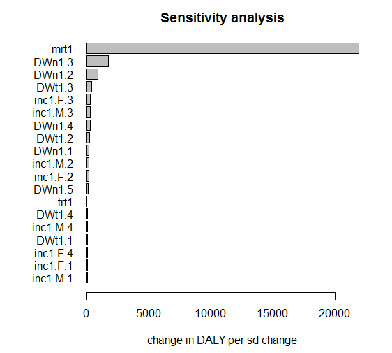
From the above results, we learn that the uncertainty in mortality rate has the highest influence on the overall uncertainty. Indeed, one standard deviation change in mortality rate would lead to a difference of more than 20,000 DALYs in the overall DALY estimate.
Further note that the names of the different input parameters are constructed as a combination of the input element, the sex (in case of sex stratification), and the age group (in case of age stratification).